
OpenCV-5 Histogram
by
본 포스트는 https://wiserloner.tistory.com/843 를 참고하여 만들었습니다.
Histogram
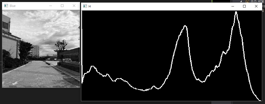
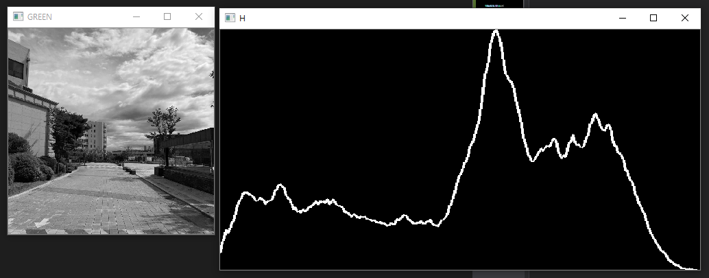
히스토그램은, 이미지의 픽셀 값의 분포를 보여주는 그래프이다.
x축은 픽셀 값의 범위(0~255), y축은 해당 픽셀 값에 속하는 픽셀의 개수 이다.
픽셀 값이 어두울수록 0에 가깝고, 밝을 수록 255에 가깝다.
calcHist 함수
calcHist 함수 : 히스토그램을 구하는데 사용됨.
void calcHist(const Mat* images, int nimages, const int* channels, InputArray mask, OutputArray hist, int dims, const int* histSize, const float** ranges, bool uniform = true, bool accumulate = false);
images = 입력 이미지의 주소
nimages = 입력 이미지의 개수
channels = 히스토그램을 구할 채널 번호. 싱글 채널이므로 0.
mask = 히스토그램 지정할 영역 지정. Mat()가 default(아무 동작 안함)
hist = histogram 결과 저장할 공간.
dims = 출력 히스토그램의 차원 수.
histSize = 각 차원의 bin 개수. 빈도수를 분류할 칸의 개수
ranges = bin의 최소, 최대 값 의미
uniform = 히스토그램 빈이 등간격인지, 비등간격인지 나타냄. 등간격일시 true, 비등간격일시 false.
accumulate = 누적플래그. 이것이 true이면 hist 배열을 초기화하지 않고 누적하여 히스토그램을 계산.
Normalize 함수
예를 들면 , 1~10 인 값들을 0~1사이 값들로 비례하게 변환해 주는 함수이다.
normalize(histogram,histogram, 0, histImage.rows, NORM_MINMAX);
첫 번쨰 인자 : input
두 번쨰 인자 : output
세 번쨰 인자 : 변환 최소값
네 번째 인자 : 변환 최대값 (히스토그램의 세로 길이)
다섯 번쨰 인자 : 변환 방식 (최소 값이 0, 최대 값이 histImage.rows 가 되도록 선형 변환)
line 함수
line(histImage, Point(bin_w * (i - 1), hist_h - cvRound(histogram.at<float>(i - 1))), Point(bin_w * (i), hist_h - cvRound(histogram.at<float>(i))), Scalar(255, 0, 0), 2, 8, 0);
첫 번째 인자 : 선이 그려질 이미지
두 번째 인자 : 선분의 시작점 (0,(hist_h - (histogram에서 (i-1에 해당하는 값)))(첫번째 선의 경우)
histogram.at<float>(i - 1) : Mat의 각 픽셀 값에 접근하는 함수. histogram의 i-1 번 위치의 data에 접근.
세 번쨰 인자 : 선분의 끝점 (bin_w*1, (hist_h - histogram에서 (i에 해당하는 값)))
네 번째 인자 : scalar . //색, 선 굵기, 선 타입 등. 정의
at() 함수 : 각 원소로 접근하기 위해 사용.
histogram.at<float>(i - 1) 에서
CODE
#include <opencv.hpp>
#include <iostream>

using namespace std;
using namespace cv;


int main() {
    // load an image
    Mat my_image = cv::imread("1.jpg", cv::IMREAD_COLOR);

    Mat bgr[3];

    split(my_image, bgr);


    MatND histogram;
    const int* channel_numbers = { 0 };
    float channet_range[] = { 0.0, 255.0 };
    int number_bins = 255;
    const float* channel_ranges = channel_range;

    calcHist(&bgr[2], 1, channel_numbers, Mat(), histogram, 1, &number_bins, &channel_ranges);

    int hist_w = 512;
    int hist_h = 400;
    int bin_w = cvRound((double)hist_w/ number_bins); //bin의 가로폭 구하기 위한 반올림

    // histImage 객체 초기화. CV_8UC1 이므로 싱글 채널, 모든 픽셀 0으로 초기화
    Mat histImage(hist_h, hist_w, CV_8UC1, Scalar(0, 0, 0));

    normalize(histogram,histogram, 0, histImage.rows, NORM_MINMAX);

    for (int i = 1; i < number_bins; i++)
    {
        line(histImage, Point(bin_w * (i - 1), hist_h - cvRound(histogram.at<float>(i - 1))),
            Point(bin_w * (i), hist_h - cvRound(histogram.at<float>(i))),
            Scalar(255, 0, 0), 2, 8, 0);
    }


    namedWindow("RED", WINDOW_NORMAL);
    resizeWindow("RED", 300, 300);
    namedWindow("H", WINDOW_NORMAL);
    resizeWindow("H", 700, 350);

    imshow("RED", bgr[2]);
    imshow("H", histImage);


    cv::waitKey(0);
    return 0;
}
결과 사진
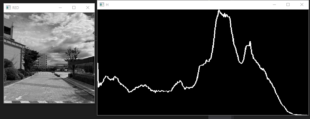
해석
Mat my_image = cv::imread("1.jpg", cv::IMREAD_COLOR);
에서는, B,G,R 3개의 채널이 결합된 멀티 채널 상태이고, 이를 3개 채널을 담을 싱글 채널 배열인 bgr[3]에 담아준다.
for (int i = 1; i < number_bins; i++)
{
    line(histImage, Point(bin_w * (i - 1), hist_h - cvRound(histogram.at<float>(i - 1))),
        Point(bin_w * (i), hist_h - cvRound(histogram.at<float>(i))),
        Scalar(255, 0, 0), 2, 8, 0);
}
에서, y 값을 plot 하는 부분에서
hist_h - cvRound(histogram.at<float>(i - 1))
구조가 잘 이해가 안갔었는데,
Mat 구조 상 좌측 상단 좌표가 (0,0), 좌측 하단 좌표가 (0, 255)임을 이용하였다.
for (int i = 1; i < number_bins; i++)
    {
        line(histImage, Point(bin_w * (i), hist_h),
            Point(bin_w * (i), hist_h - cvRound(histogram.at<float>(i))),
            Scalar(255, 0, 0), 2, 8, 0); //색, 선 굵기, 선 타입 등.
    }
의 결과 사진을 보면 직관적으로 알 수 있다.
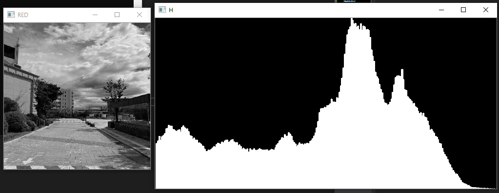
시작 좌표인 Point(bin_w * (i), hist_h) 에서, y 좌표가 hist_h 이므로 좌측 하단부터 시작, 끝 좌표 Point(bin_w * (i), hist_h - cvRound(histogram.at<float>(i))) 에서 y좌표를 통해 좌측 하단으로부터 떨어진 정도를 볼 수 있다.
Subscribe via RSS